What is convergence?

In the previous post on stability, we saw a few familiar properties that indicate stability in the system. However, what we really mean when we are looking for stability is a system that is robust to small rounding errors. In other words, we want convergence.

By exploring fixed points, we will be able to properly define what this means, and build an intuition for what convergence looks like.

Before we start

In the post on chaos, we covered the definition of a dynamic system. For our purposes, a dynamic system is that it is a function that iterates repeatedly, with the output becoming the input for the next timestep.

Just to make our lives easier, let’s use the notation $f \circ f(x)$ to mean $f(f(x))$.

Fixed points

Fixed points are really simple: they are inputs that are unchanged by the function. For example, $0$ is a fixed point of $x^2$ since $0^2 = 0$. Here’s another few examples:

1. In $y = x$, every point is a fixed point.
2. In the logistic map $3.95 \cdot p \cdot (1 - p)$, 0 is a fixed point.
3. 100% is the fixed point of charging your phone.
4. $0 is the fixed point of earning interest.

The formal definition of a fixed point is:
If $f(x) = x$, then $x$ is a fixed point for the function $f$.

The four examples listed above actually exhibit different types of fixed point dynamics. As we learn about the different types, we will use these examples to show the differences.

Red herring: Attracting fixed points

This type of dynamic has a very simple definition: not only does an attracting fixed point $x$ map to itself, but at least one other point is mapped to $x$ as well. More formally, we have $f(x) = x$, and in addition, there exists some other point $y$ such that $f(y) = x$.

So far, attracting fixed points look pretty promising to help us define convergence. Not only do they stay fixed, but other inputs can end up at this result as well (hence attracting). Intuitively, this sounds like convergence, with multiple inputs leading to the same output.

Let’s see how it plays out in our examples, and whether this is a good enough definition of convergence:

1. $\ f(x) = x$: Every point is a fixed point, but none of them are attracting.
2. $\ f(p) = 3.95 \cdot p \cdot (1 - p)$: 0 is an attracting fixed point, since $f(1) = f(0) = 0$.
3. Phone charging: 100% is an attracting fixed point. Charging from 99% gives 100%.
4. Earning interest: $0 is not attracting. You can’t earn interest from some money and end up with no money.

These examples are just all over the map.

Some systems, like earning interest, really feel pretty stable, but aren’t attracting. The logistic map in example 2 is completely wacky. It has an attracting fixed point, but in the chaos 101 post, we saw that it is actually chaotic almost everywhere else.

The confusion is that attracting fixed points are stable for points that converge to them, but aren’t sufficient for stability of the rest of the system.

We need something stronger…

Convergence for engineering

There’s a bunch of different mathematical definitions of convergence. A lot of them depend on how quickly the system converges, or differentiate between converging to a point and just getting really close.

From an engineering perspective, there are only three bounds that matter:

• $N$: our “sufficiently large” number. We often choose an upper bound for how large we care to check. This upper bound can be an order of magnitude, or maximum number of iterations that make sense in our system.
• $\varepsilon$: This is our margin of error. This is basically asking how wrong is actually still ok in our system.
• Expected input: in engineering, the behaviour of the system in general does not matter. The only thing that matters is the behaviour on expected input.

Armed with $N$, $\varepsilon$, and our inputs, we can define convergence for engineers:
A system is stable on the expected input if two points that are within $\varepsilon$ of each other stay within $\varepsilon$ of each other after $N$ iterations. These two points must be from the expected set of inputs.

Formally: Let $U$ be our set of inputs. $f$ converges for engineers if for $x, y \in U$ and $|x - y| \lt \varepsilon$, we have $|f \circ f \circ \dots \circ f(x) - f \circ f \circ \dots \circ f(y)| \lt \varepsilon$.
Recall that $f \circ f(x) = f(f(x))$.

Let’s look at our four systems, and which ones converge from an engineering perspective:

1. $f(x) = x$: Definitely converges. Two points that start off close together stay close together because … well … they just don’t move.
2. $f(p) = 3.95 \cdot p \cdot (1 - p)$: Here it really matters what the possible inputs are. If we know for a fact that we only put 0 or 1 as an input, then sure, it converges. But, if we are choosing input from around 0.3, as we know, the system is chaotic.
3. Phone charging: Converges! Eventually all points end up at 100% anyway, and points stay close together over time.
4. Earning interest: Here is where we REALLY care about $N$. Normally, the same input doesn’t earn interest for millions of iterations. Moreover, there are usually upper bounds on the inputs. Even though earning interest is exponential, if you know you won’t have more than a couple thousand iterations, you can easily check which inputs have acceptable error margins. The same small rounding error matters less if the input was 3 than if it was 3 billion.

Fixed points: Useful after all

Let’s take a look at gradient descent, which follows the slope downwards to find the local minimum. Let’s see how gradient descent behaves on $x^4−x^2$.

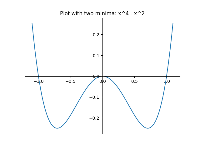
If you start with $x \gt 0$, no matter what, through gradient descent you will end up at the fixed point $x = \frac{1} {\sqrt{2}}$. Similarly, gradient descent from $x \lt 0$ will always result in $x = - \frac{1} {\sqrt{2}}$.

But what about $x = 0$? The derivative here is 0, so there isn’t a natural “descent” in one particular direction. Basically, this point is the boundary between two regions that converge to different points. Near zero, the system is highly sensitive to the input conditions: slightly above or below 0 give totally different answers.

What can we learn here from fixed points?

Let’s look at our three points with derivative 0.

Two of them are the local minima we are looking for. In terms of the dynamics, the two minima are attracting fixed points, and also points that the system converges to. Since the system converges almost everywhere to one of two points, allowing a pretty large error would result in the same answer in most cases.

The maximum at $x = 0$ is not a convergence point. It isn’t even an attracting fixed point; unless we start at $x = 0$ we will never accidentally end up there.

However, it is the boundary between two regions that converge to different points. There is a small neighbourhood around $x = 0$ where a change in the tiniest $\varepsilon$ could flip the input from negative to positive. All of a sudden, the “inconsequential” error margin completely changed the output. This is crucial information.

We’ve seen this behaviour before. The fixed point of $0 in earning interest is the difference between earning money and sinking into debt. In the logistic map if the input is less than 0, then the output doesn’t end up inside [0, 1], instead it flip flops between positive and negative, and approaches infinity.

Even when fixed points are not convergence points, they can give us excellent hints about the behaviour of the system, and more importantly, boundaries between different system behaviour.

Bottom line

From an engineering perspective, the behaviour of the system only matters on the expected input. Moreover, if the system stays within an appropriate error rate for a reasonable number of iterations, it really does not matter at all if the system is completely chaotic in other conditions.

Testing all possible expected inputs is usually not possible. Luckily, fixed points are often significant to the system’s behaviour, and can give us a lot of insight into the dynamics. We may discover that a particular fixed point is a convergence point or a boundary between different system behaviours.

What’s next?

In the last few posts, we’ve covered behaviours of systems in a general sense, and seen some small examples that exhibit these behaviours.

The next step is to ask about more complex applications, and how to test them for local dynamics and chaos. This is particularly important for HPC applications.

I’ll also cover common sources of error due to floating point representation.