Chaos 101: a small change in input is a BIG change in output

Many systems are chaotic.

Some are only interesting to physics classes, like the double pendulum. Some, like the three-body problem, are concrete physics problems that feel a bit more important. However, the weather is also a highly chaotic system, and the fact that weather prediction is so complex has an immediate effect on all of our daily lives.

We’ve all seen the infamous “30% chance of rain” and felt completely clueless about how to dress. More importantly, if we could accurately predict serious natural disasters like hurricanes and tsunamis, we could make effective plans, save crops, and even save lives.

Chaos is rigorously mathematically defined. The definition is concise and accurate. But … it’s not particularly easy to understand. We’ve all heard of the “butterfly effect”, but despite the vivid imagery, understanding chaos remain elusive.

I will first walk through the mathematical definition in plain English, and then use some easy examples to build an intuition for what chaos is and what it looks like.

When close enough ISN’T good enough

Let’s start with an easy example: $f(x) = \frac{1} {x}$, and an error of $10^{-6}$.

If I choose $x = 0.00001$, then $\frac{1} {0.00001} = 100,000$. So far so good.

But what if I add $\varepsilon = 10^{-9}$ to the input? Unfortunately, then $\frac{1} {0.00001 + \varepsilon} \approx 99,990$. Yikes. My output changed by 10. It was just the tiniest difference in input, but it left my error tolerance in the dust.

On the one hand, yeah, don’t divide by zero (or really close to zero). Isn’t that the only math rule anyone ever cares about?

Ideally, after this post, there will be at least one more math rule that you care about. The idea is to show that this type of unexpectedly drastic change in output isn’t isolated to dividing by zero.

What is a dynamical system?

A dynamical system is just a function that evolves a system over time. Any timestep function is a dynamical system, where the system at time $t$ is dependent on the system at time $\lt t$, and ultimately the starting conditions.

Formally, a dynamical system is a function where the range is equal to the domain. In other words, the output can become the “starting conditions” for the next iteration.

Since computers can only do discrete calculations, scientists often model continuous systems with discrete systems. Some examples are weather forecast, molecular dynamics simulations, double pendulums, most ordinary differential equations (ODEs).

Why does this definition matter? It matters because of chaos.

What is chaos?

Some dynamical systems are chaotic: they are extremely sensititve to initial conditions. This is what we saw with $\frac{1} {x}$ near zero. A miniscule rounding error can change the output drastically. However, this isn’t the worst case scenario. At least $\frac{1} {x}$ is well behaved – the function changes in the same direction. If my answer is way larger than expected, at least I know my error was to round down.

If a system is mixing, the teeniest change in the input of $\varepsilon$ can have ANY effect on output – no matter how tiny the $\varepsilon$ I choose is.

Let’s start with the formal definition of “mixing”, and walk through it with an example.

Mathematical definition: topological mixing

A system is topologically mixing if for every two open sets $U$ and $V$, there is a time $t$ of the system such that $U$ iterated $t$ times intersects (overlaps with) $V$ iterated $t$ times.

This implies that if you allow a change in your input by $\varepsilon$, no matter how small, your output after a bunch of iterations could be anywhere. Essentially, it’s the butterfly effect. Let’s look at an example of this to understand what this looks like.

Disclaimer: A crucial part of this defintion is the open set. In the following example, we will see a visual demonstration of this type of chaotic dynamic, but keep in mind that this example is over a finite input set.

Example of chaos and mixing: logistic maps

The logistic map is a class of functions of the form $r \cdot p \cdot (1 - p)$, where $p$ is between 0 and 1 inclusive. For this example, let’s choose $r = 3.95$ (yes, this is a very intentional choice).

Essentially, we have two sets of 200 densely packed points as the starting conditions: one set between $[0.3,\ 0.301]$ and one set between $[0.8,\ 0.801]$. There was no particular reason for those values. Due to the chaotic nature of this function, we would see a similar effect with any two input sets.

These sets are graphed at $t = 0$. For $t = 1$, each point was mapped through the map $logisticMap(p) = 3.95 \cdot p \cdot (1 - p)$. Similarly, to get the points at $t = i$, I simply mapped all the points at $t = i - 1$ through the logistic map.

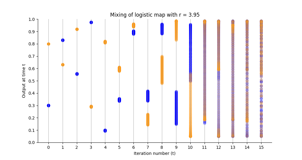
What are we looking at here? Let’s walk through this.

At $t = 0$, we see the starting conditions as described above, colour coded. Even though I plotted the points with low opacity of 0.2, we see solid blue and yellow dots since the individual dots are so closely packed on top of each other.

For the first few iterations, we see what we expect to see. The dots start out close together, and are mapped around together, staying closely packed.

At $t = 5$ we start to see for the first time that the sets are slightly more spread out than they were previously, and from $t \gt 5$ the dots start to spread out significantly.

At $t = 10$ we see the first iteration that satisfies the definition of mixing – all disjoint open sets are eventually mapped to an overlap.

But, just for funsies, I included the next few iterations as well, where we see the significance of a mixing dynamic. What we see in $t \gt 10$ is the more intuitive understanding of chaos – the blue and yellow sets end up basically everywhere.

This shows why this type of dynamic is called mixed. No matter which set you choose, or how tightly packed it starts, eventually, after enough iterations the set will be fully “mixed” into the system. Just like a drop of food colouring in a glass of water.

I posted the code that generated this figure here.

Exercise for the reader:

1. Prove that if $0 \lt p \lt 1$ and $r = 3.95$, then in the logistic map $\quad f(p) = 3.95 \cdot p \cdot (1 - p)$, we have $0 \leq f(p) \leq 1$.
2. Prove the same thing for all $0 \lt r \lt 4$.

The bottom line

We now understand dynamic systems, and have seen an example of chaos and mixing. What we’ve also seen is that in these systems, a tiny change to the input can have basically any effect on the output. Moreover, I was able to create a highly chaotic system with only three compute operations – two multiplications and one subtraction. I didn’t have to construct some crazy looking ODE.

This is extremely crucial to understand. The “close enough is good enough” philosophy of rounding is so prevalent, especially since it is impossible for a computer to have perfect precision. Yes, a lot of the time we really are in non-chaotic systems, and a teeny bit of rounding is completely safe. However, in a chaotic system, this is simply not the case, and it is definitely worth confirming that a “negligible” rounding error is in fact inconsequential.

What’s next?

Many systems are chaotic … but luckily many aren’t. In future posts, I will cover other dynamics.

I will also post about rounding errors in floating point arithmetic that can cause some funky behaviour in a chaotic system.

Throughout the chaos series, I will continue to use the logistic map with different $r$ values as examples. I will include an engineer-friendly post, but there’s also some pretty great content on Wikipedia.